Introduction

A number of times over the past three years I've had trouble with a KVARZ CH1-76 Passive Hydrogen Maser (PHM). Although the maser has never failed catastrophically, the symptoms range from dramatic drops in short-term stability, to phase jumps, to periods of long-term instability. It is possible more than one problem exists. It is clear the problems are infrequent and intermittent.

The CH1-76 internal diagnostics are very limited: error code 1 is sometimes displayed and correlates well with a reduction of short-term instability; error code 4 is present much of the time on this H-maser, but doesn't appear to correlate with stability problems (confirmed with the factory). The symptoms appear to be uncorrelated with temperature, voltage, orientation, or the phase of the moon.

Anyway, after what happened last week, today seems to be a good day for the maser. I am writing this note to serve as a baseline to help identify trouble in the future.

TSC 5110A plots

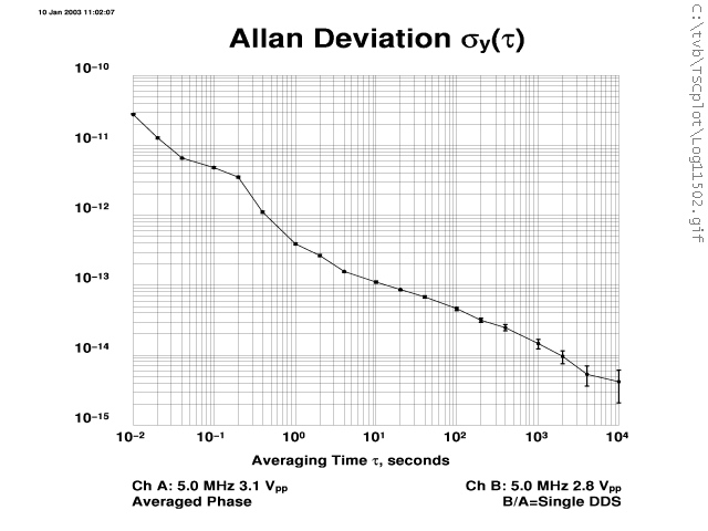
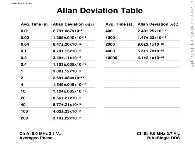
The following four TSC 5110A screen shots were taken about 11 hours into a run. That's 40,000 seconds; the point where the Allan Deviation, s_y(t), for tau, t, 10,000 seconds appears on the real-time display. A stability of 4E-15 at 10k seconds is pretty good for the passive maser. Already I can tell this will be a good run.

Remember that any phase detector, frequency counter, or Time Interval Analyzer (TIA) like the TSC 5110A produces phase or frequency difference measurements and thus the stability plots are a function of both the source and the reference. Usually one selects a reference that is known to be at least 10x better than the source in which case the plots can view viewed as essentially absolute measurements.

The frequency reference for this run is a KVARZ CH1-75 Active H-maser (AHM) which, so far, is working flawlessly. At this point I don't know exactly how much better the AHM is but other measurements I've taken suggest that any limits in the plots below are due to the PHM source rather than the AHM reference. The short-term stability of this AHM is much better than a 5071A cesium standard which is why I like to use it as a reference.

AHM (CH1-75) vs. PHM (CH1-76) after 40,000 seconds

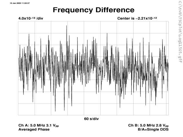
The Frequency Difference plot shows the stability for the previous 9 minutes. One gets a feeling for short-term stability from 1 to about 500 seconds. The PHM is low in frequency by 2.21E-12 relative to the AHM. Based on previous measurements this is likely due to an accumulation of months of drift. The maser has been operating here for three years and masers do drift. If, for example, the daily drift rate were consistently 5E-15, the net frequency error would be about 30 x 5E-15 = 1.5E-13 per month, or 1E-12 after six months. This gives you an idea why a maser might be "this far off" in frequency over the years. Then again, this drift rate is 100,000 times less than a HP 10811A oscillator!

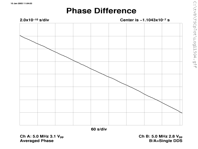
The Phase Difference plot above is uninteresting. This is due to the fact that the TSC 5110A, in single DDS mode, plots raw phase rather than frequency corrected phase. If a linear phase drift (i.e., frequency offset) were removed the plot would be more revealing. When a sufficiently large frequency offset exists any auto-scaled phase plot will be a straight line from corner to corner. In this case the slope is about -6 x 2E-10 / 9 x 60 = -2.2E-12 which agrees with the center frequency shown on the Frequency Difference plot.

Stable32 plots

The TSC 5110A produces wonderful, simple, real-time plots. When the raw 1 Hz phase data from the TSC 5110A serial port is logged to a PC additional analysis can be done off-line with tools such as Stable32. The raw data for the 40,000 second run (480 kB) looks like:

-0.1183169
-0.1183246
-0.1183379
-0.1183488
-0.1183565
...

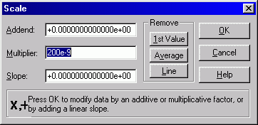
Some instruments produce phase data in units of seconds, or microseconds, degrees, or radians. The TSC 5110A serial output is in units of the period of channel A. With a 5 MHz frequency input the period is 200 ns so we would multiply each reading by 200e-9 to get time interval in seconds.

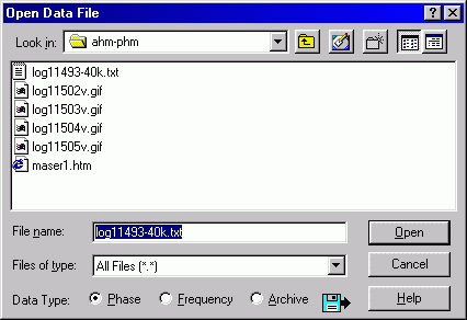
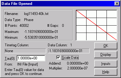
I'm including detailed Stable32 screen shots below; partly to remind myself how to use it and partly as a mini-tutorial for the reader. Click on File->Open and remember to choose "Phase" data rather than "Frequency" as the type of data:

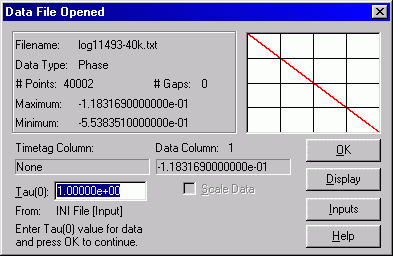
Next, the tau value for the data must be given. The TSC data rate is 1 Hz which is conveniently the Stable32 default:

Now, the raw phase data needs to be scaled. There are two ways to accomplish this. One way is to use Edit->Scale and enter the 200 ns scale factor:

The other, and perhaps easier, way to scale the data is to use the Inputs and Scale Data buttons which are part of the open dialog itself:

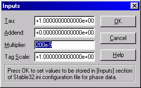
The tau and scale factors are "sticky" so next time you run Stable32 they will be the defaults:

Finally, use Plot->Phase to generate the following:

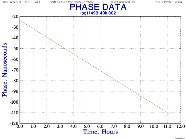
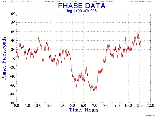
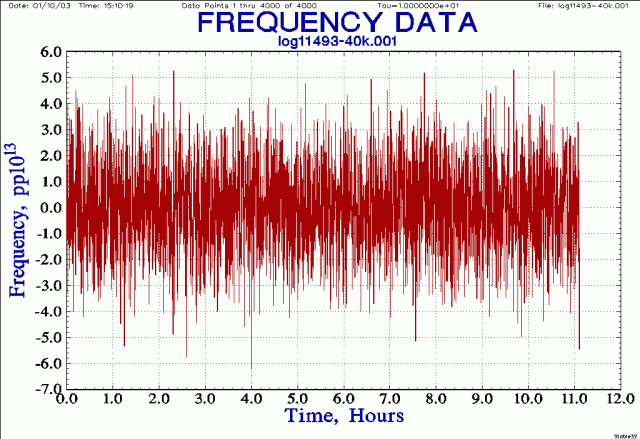
The plot shows the entire 11 hour phase record not just the most recent 9 minutes (as with the TSC 5110A). As expected, the plot is a negatively sloped very straight line. The phase is decreasing meaning Channel A is catching up with Channel B. In terms of frequency this means channel B (PHM, source) is slow relative to channel A (AHM, reference). As noted earlier, the slope of the line indicates a frequency offset and the smoothness of the line simply indicates the noise is hidden by the scale of the graph. The slope is approximately -90 ns / 11 hours = -2.2E-12.

The fact that there is a frequency offset is not of great interest in this case. Offsets can be corrected using the front-panel synthesizer setting, an external phase microstepper, or in software. Since neither the phase offset nor the frequency offset has any effect on the computed Allan Deviation they can be mathematically removed. In practice, since I'm more interested in stability than accuracy, it is easiest to remove offsets in software rather than making physical adjustments to a running maser.

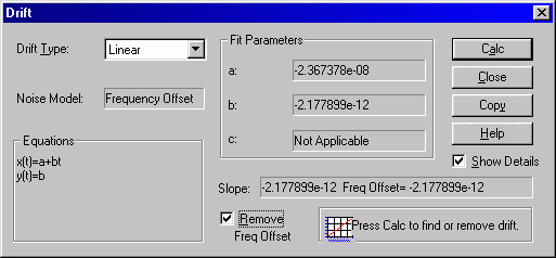
Use Analysis->Drift to compute the linear drift (i.e., frequency offset) from the phase data. Now that we know the frequency error is -2.177E-12 we can go ahead and remove it:

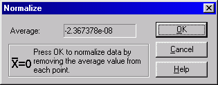
The above dialog only removes the frequency offset so use Edit->Normalize to remove the phase offset:

With the phase and frequency offsets removed we get our first clear view of the noise remaining. The resulting residual phase plot shows two masers keeping time to within 150 ps over half a day:

Ok, now it's time to see the frequency domain. We do this using Edit->Convert to convert from phase to frequency:

Here is a frequency domain plot:

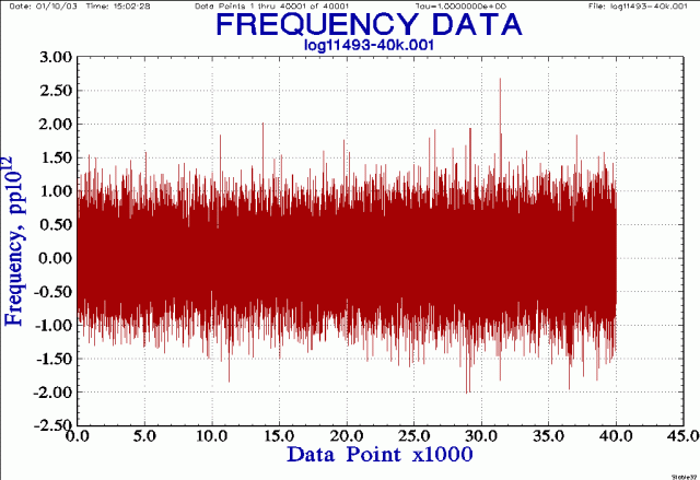
This looks like a flat line (no apparent frequency drift). Each point represents a 1 second frequency measurement. The noise is about 2E-12 peak-to-peak. To reduce the noise use Edit->Average to average the readings, removing some of the white noise:

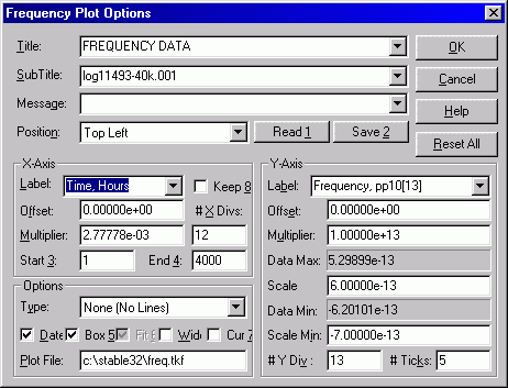
Also while we're at it use Plot->Frequency->Options to change the default x-axis scale from points to hours and set X-divs to 12 so each grid line is 1 hour:

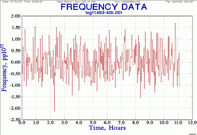
The resulting plot is then based on 10 second frequency averages. The noise is about 10E-13 peak-to-peak.

An additional 10x averaging gives this frequency plot with 100 second averaging:

And finally, with 1000 second frequency averages we get this plot:

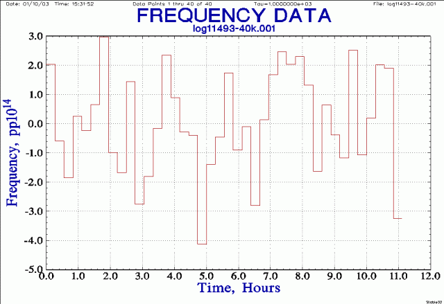
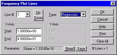
We see the two masers, at 1000 seconds, are stable in frequency to a few parts in 10¹⁴th. Stable32 will compute the slope (i.e., frequency drift), if any, of this frequency data. Use Plot->Frequency->Lines to best fit a line through this data:

And then plot it:

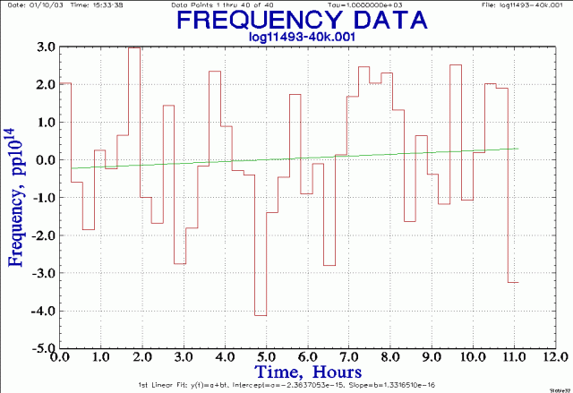
Although the line has a non-zero slope the data is so ragged at this scale that no conclusion should be drawn from the drift line. The slope looks about +0.5E-14 over 11 hours, or 1E-14/day. The calculated slope is 1.33165e-16 which is in units of 1E-14 per 1000 seconds (due to the averaging), or 1.15E-14/day.  But I would not want to state what a maser's drift was until the drift line rose well above the noise; this could take days or weeks of data. As you can see above, half a day of measurements is still noise compared with maser drift rates.

Use Analysis->Run to generate the Allan Deviation plot:

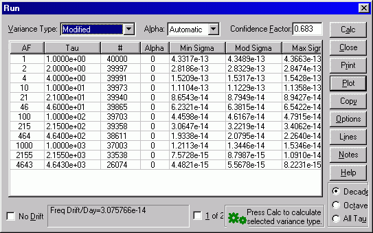
We'll use Modified Allan Deviation here:

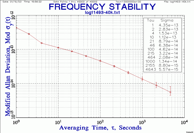
Even though I used a data set of 10,002 phase points Stable32 doesn't calculate the sigma at tau 10⁴ in decade mode. So one can use All Tau mode instead (though it takes forever to calculate and plot):

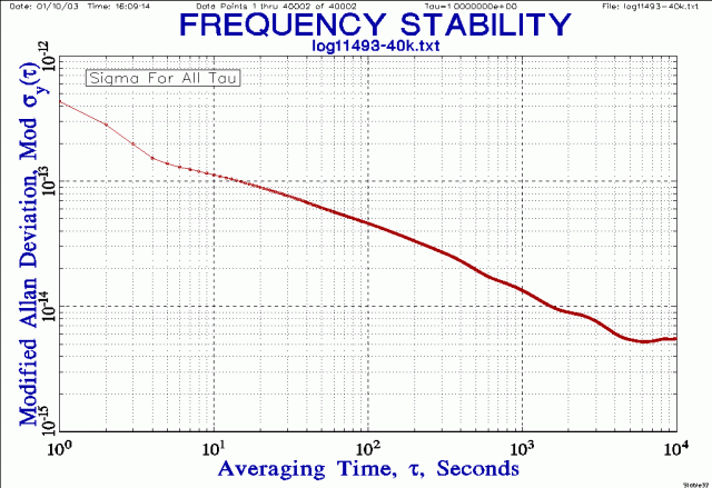
Already from this plot we get a hint that the passive maser hits a floor at about 5E-15.

Conclusions

The maser is working fine for the first half-day of this run. There is a danger in believing statistics when the sample size is insufficient. This is especially true with Allan Deviation for large tau, where the sample size is almost always less than you'd like. It is also inappropriate to blindly calculate daily drift rates without looking first at the plots to see if there is a valid trend or not. Equations will always produce a result; but the result can be bogus.

In a few days, we'll take a fresh look at how the maser is doing.